Excel is a well-known powerhouse that most everyone has used at some point in time. While Excel is such a popular tool, not to mention the world’s premiere spreadsheet application, it is pretty rare that you find someone that is proficient in it. Most people probably don’t even know all of Excel’s capabilities. Below are a few tricks for Excel that may make your life a little easier when trying to use the program.
1. Line Breaks and Wrapping Text

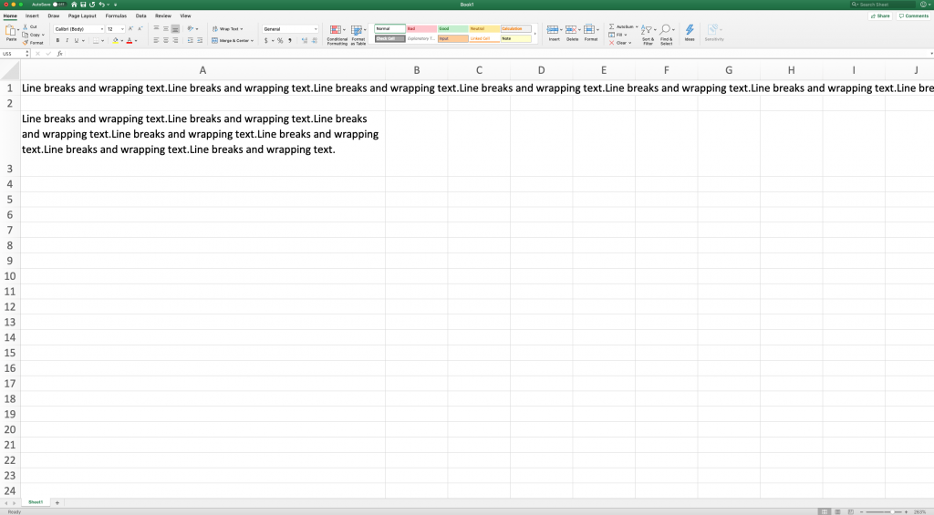
The default of Excel is for the text to run forever as you type. This can be frustrating, as the line of text never wraps around to a new line. There is a way to fix this. You are able to create a new line by typing Alt+Enter, or you can click the Wrap Text button under the home tab of the screen. This option allows you to type into a single cell and the text wraps to the next line automatically when it hits the edge of the cell. When a row or column is resized, the text re-wraps to fit.
2. Multiple Cells, Same Data
If, for some reason you need to type the same thing over and over again in multiple cells in a worksheet you can do this by selecting all the cells you wish to display the data in. You have the ability to select entire rows or columns, multiple single, seemingly random cells, or anything in between. In the last cell selected, type in the data and hit Ctrl+Enter. Your text should appear in each cell you selected.
3. Ctrl+Shift to Select

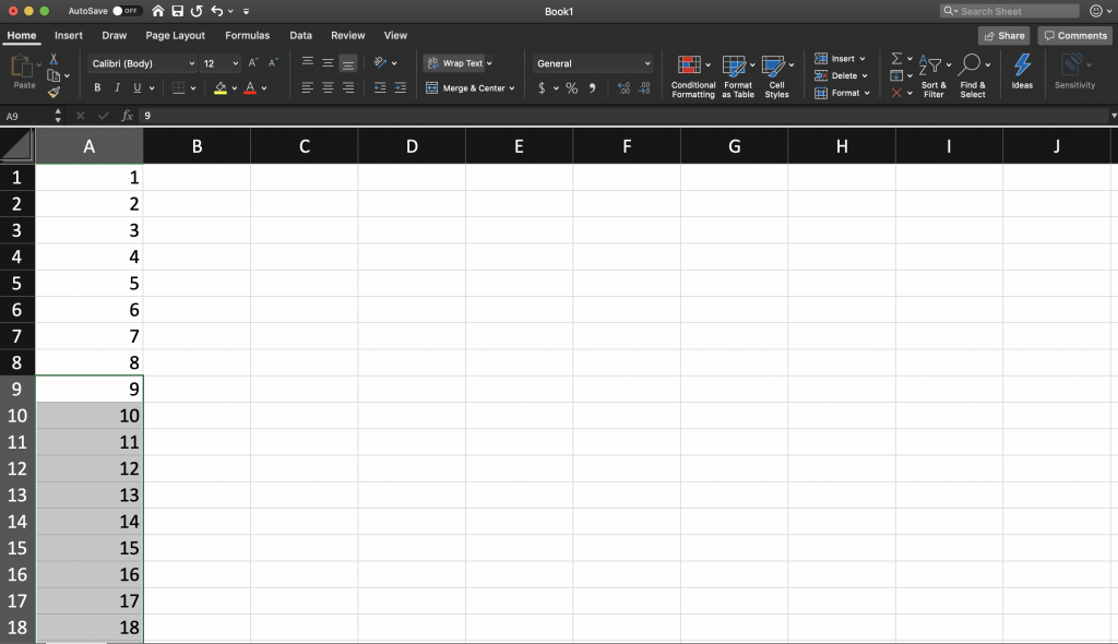
A shortcut to selecting multiple cells in a row and/or column, click in the first cell, hold Ctrl+Shift and the down or up arrow (depending if you would like to select the data in the column above or below the cell selected initially), or the left or right arrows (if you would like to select the data in the row to the left or right). You can hit multiple arrow keys (up, down, right, and/or left) to select an entire row, and entire column, or both.
If you would like to only select cells with data, you can use Ctrl+Shift+End. First select the cell where you would like the data selection to begin, then hold the before specified keys. This will send the cursor to the lowest right-hand cell that contains data, selecting everything in between. If you would like to select absolutely everything on the worksheet, you can use Ctrl+Shift+*.
4. Use Graphics in Charts
You are able to put graphics in any element of an Excel chart. To put a graphic in a piece of pie on a pie chart, bar graph, etc., use the Series Options fly-out menu and select “Picture or texture fill”. To achieve a missing pie slice, you are able to select “no fill”
5. Auto Fill
For typing repetitive sequences such as dates, you can begin the series and move the cursor to the lower-right corner of the last cell, which is currently selected. When the cursor turns into a plus sign, click and drag down the column or across the row, whichever way highlight the cells where you intend for the sequence to continue.
6. Flash Fill
If you start typing a pattern, Flash Fill will automatically recognize the pattern and fill in a column based on the data it sees in the first column. For example, if the first column of your worksheet contains phone numbers that are not formatted (ex: 1234567890) and you would like them to be formatted, (ex: (123)456-7890), begin typing that formatting in the first few cells. After the second cell, Excel should recognize the pattern and start suggesting formatting. In order to use the suggested formatting, simply hit the Enter key on the keyboard.
7. Save Charts as Templates
Excel has many charts as defaults to use. However, it can be nearly impossible to find a chart that fits your needs. Luckily, there are many options for editing charts in order to make it fit your needs. You may spend a lot of time tweaking your chart to be exactly how you would like it. But how about when you wish to recreate the same chart? It’s likely you may not want to go through all the same steps again. Thankfully, you don’t have to because you are able to save a chart as a template.
Once you have a chart exactly as you wish it to be, right-click it. Select Save as Template. Save the template with a CRTX extension in the Chart Templates folder.
To apply the chart template you created to a chart, all you need to do is select all the data in the chart, go to the Insert tab, click Recommended Charts, and then the All Charts tab, then the Templates folder. Select the template you would like to apply from the “My Templates” box. To finalize the application, click OK.
A chart template is able to apply font, color, embedded graphics, and series options. However, it will not translate other elements such as the actual text in the legends and titles.
8. Text to Columns
If you would like to change one column into two, you can do that easily without re-typing anything whatsoever. For example, if you have a list of full names (first and last), you are able to break the first names apart from the last and make two different columns for them.
To do this, select the data, go to the data tab, and click Text to Columns. A window should appear asking if you would like to separate the words by the delimiters (spaces or commas), or by a fixed width. Select one and click OK.
9. Conditionally Format
Excel’s conditional formatting is helpful when needing to quickly identify the highlights. Who has the highest or lowest score? What are the top five? From the Home tab, click Conditional Formatting. A pop down menu will appear from which you may click New Rule. Input your preferences, and click OK. You can also create more rules within other options in the drop down menu like a rule to look for things like a string of words, recurring dates, or duplicate numbers.
10. Hide a Worksheet
Often, when you’re working in a workbook, it may become cluttered with many different worksheets. You may have a worksheet that you use, but that doesn’t necessarily need a place in the worksheet tabs at the bottom of the screen. An example of a sheet that you may want to hide but not delete would be a sheet with formulas, or references. In order to hide a sheet, right-click the bottom sheet tab and select Hide. When you need to view the sheet again, go to the top “View” tab, click Unhide, and pick the sheet name from the list that pops up.
